Trophic state: OECD boundaries and the LAWA index
Trophic state describes the nutrient supply and thus the productivity of a water body. In 1982 the OECD published fixed class boundaries that still carry international understanding today.1 They rest on three quantities found in every monitoring programme: total phosphorus, chlorophyll-a as a measure of algal biomass, and Secchi depth.
Class boundaries according to OECD (1982), annual means| Stage | Total phosphorus | Chlorophyll-a | Secchi depth |
|---|
| oligotrophic | below 10 µg/l | below 2.5 µg/l | above 6 m |
| mesotrophic | 10 to 35 µg/l | 2.5 to 8 µg/l | 3 to 6 m |
| eutrophic | 35 to 100 µg/l | 8 to 25 µg/l | 1.5 to 3 m |
| hypertrophic | above 100 µg/l | above 25 µg/l | below 1.5 m |
In Germany, the federal-state working group on water (LAWA) assesses lakes by the trophic index (LAWA 2014).2 It combines the same three quantities in a lake-type-specific way and distinguishes eight classes from oligotrophic to hypertrophic, including two polytrophic stages that the OECD scheme lacks. The animation follows the four stages from oligotrophic to hypertrophic according to the OECD scheme, which additionally recognises an ultra-oligotrophic class below them, because it is internationally comparable and its boundaries translate directly into model values.
Of the three quantities, Secchi depth is the oldest: a white disc on a line, lowered until it disappears. Carlson built his Trophic State Index on it in 1977 because Secchi depth is available everywhere and without instrumentation.3 It is a summary measure of algae, suspended matter and dissolved humic substances4 and therefore a robust but not a fast indicator: it shows what is already suspended in the water.
Phosphorus is the lever
That phosphorus, not nitrogen or carbon, limits algal growth in lakes has been established since a whole-lake experiment in the Canadian Experimental Lakes. In the early 1970s, Schindler divided Lake 226 with a plastic curtain: one half received carbon and nitrogen, the other additionally phosphorus. Only the phosphorus half developed a cyanobacterial bloom.5 Since then, eutrophication strategies have targeted phosphorus first, from phosphate-free detergents to phosphorus precipitation in wastewater treatment plants.4
Phosphorus reaches a lake from its catchment: through run-off from fertilised land, through erosion, wastewater treatment plants, stormwater sewers and drainage. Part of it is taken up by algae, sinks with them and accumulates in the sediment. There it is not gone, but stored. How firmly is decided by oxygen.
The cascade: stratification, depletion, release
In summer, a sufficiently deep lake stratifies: on top lies the warm, well-mixed epilimnion, below it the cold hypolimnion, between them the thermocline. For months there is hardly any exchange between the two. The deep water no longer receives oxygen, neither from the air nor from photosynthesis, which does not take place in the dark. Everything that sinks from above is broken down by bacteria at the bottom, and this decomposition consumes oxygen. The more algae grow at the top, the more biomass sinks, and the faster the oxygen at depth is used up.
The decisive step takes place at the boundary between sediment and water. Mortimer described it in 1941 at Esthwaite Water in the English Lake District.6 As long as oxygen is present at the sediment, iron exists as a trivalent oxide and keeps phosphate bound. When oxygen falls towards zero, it is reduced to the divalent, soluble form, the bond dissolves, and phosphate passes into the water. The technical term is internal loading, or phosphate release from the sediment.
With the autumn turnover, the released phosphorus is distributed throughout the water column and is available to the next generation of algae the following spring. More algae, more sinking biomass, anoxia that sets in earlier and lasts longer, more release. That is the feedback that turns a linear nutrient problem into a cascade. In shallow lakes, the summer release from the sediment can exceed the input from outside.7
Two mechanisms lead to fish kills, and they need to be distinguished.4 In deep lakes, cold-water species lose their summer refuge because the hypolimnion becomes oxygen-free. In shallow, productive lakes, oxygen collapses throughout the water column when respiration and decomposition continue on warm nights but photosynthesis does not. Both have the same cause but appear in different places and at different times, and a morning grab sample misses both.
From the eutrophic stage onwards, the question of toxins arises for bathing waters and drinking-water reservoirs. Many cyanobacteria produce microcystins. The WHO gives 1 µg/l as the lifetime guideline value in drinking water and 24 µg/l for bathing waters;8 the German Drinking Water Ordinance (TrinkwV 2023) sets a limit of 1 µg/l for microcystin-LR, applicable from 12 January 2026.9
Why response comes too late: two stable states
The idea that a lake responds in proportion to its nutrient load has been refuted for shallow lakes since the 1990s. Scheffer et al. showed that two alternative states can be stable under the same nutrient load.10 One is clear, with submerged plants that hold the sediment in place, bind nutrients and shelter the zooplankton that graze the algae. The other is turbid: phytoplankton takes the light from the plants, fish decimate the zooplankton, and the unprotected sediment is stirred up with every wind. Each of the two states stabilises itself.
The transition between them is not a dial but a tipping point with hysteresis: the nutrient load at which a clear lake turns turbid lies well above the load at which a turbid lake becomes clear again.11 Anyone who returns the input to its pre-tipping value does not get the old state back. They must go further below it, and they must wait.
How long is shown by an analysis of 35 lakes in Europe and North America where external phosphorus input was substantially reduced: in most cases the phosphorus content of the water reached a new equilibrium only after 10 to 15 years, because the sediment kept supplying it for that long; biological recovery followed with a further delay.12 During this time, water-body maintenance bodies are left with interventions in the lake itself: phosphate precipitation, aeration of the deep water, sediment removal, biomanipulation. Each of them works against a system that defends its state.
Warming shifts the thresholds
The cascade now runs under different conditions than in the decades when the class boundaries were set. An analysis of 45,148 oxygen and temperature profiles from 393 temperate lakes shows a decline in dissolved oxygen since 1980 of 5.5 % in surface water and 18.6 % in deep water.13 At the surface, the loss is explained mainly by lower solubility in warmer water. At depth, it is linked to stronger and longer-lasting stratification and to declining water clarity, precisely the quantities that control the release.
Warmer water also favours cyanobacteria over other groups of algae: they grow faster at high temperatures, regulate their buoyancy and, on calm, warm days, form the surface scums that trigger bathing bans.14 A lake that was stably mesotrophic thirty years ago under the same nutrient load can be eutrophic today without anything having changed in the catchment.
Greenhouse gas: the factor of six, derived
A tipped lake is not only a local problem. In the oxygen-free sediment, the sinking biomass gives rise to methane, which reaches the surface as bubbles or in dissolved form. In 2018, DelSontro, Beaulieu and Downing assembled the largest dataset to date on greenhouse-gas fluxes from lakes and impoundments and showed that emissions covary with the size and trophic state of the water bodies.15 Scaled up, lakes and impoundments worldwide emit 1.25 to 2.30 Gt of carbon as CO₂ equivalent per year, nearly 20 % of fossil CO₂ emissions; around three quarters of this climate effect are due to methane.
The factor of six does not come from a measurement at any particular lake but from the regression in that study: methane emission grows with chlorophyll-a according to log₁₀(CH₄) = 0.778 · log₁₀(Chl-a) + 0.940, with emission in mg CH₄-C per m² and day and chlorophyll-a in µg/l. Between the oligotrophic and the hypertrophic class boundary of the OECD, 2.5 and 25 µg/l, lies one order of magnitude of chlorophyll-a, and 100.778 is 6.0. With 1.5 and 40 µg/l, the model lake of the animation reaches further into both classes; for it, the same regression gives roughly thirteen times, and that is what the display shows. The scatter around this line is considerable. The factor describes a trend across many lakes, not the balance of a single one.
A year later, the same authors extended the calculation into the future: if the eutrophication of lakes increases over the current century to the extent that population growth, fertilisation and warming suggest, their methane emissions will rise by 30 to 90 %.16 Two findings from the Leibniz Institute of Freshwater Ecology and Inland Fisheries (IGB), which conducts research at Lake Stechlin, shift the picture once more: methane also forms in the oxygen-rich surface water of clear lakes,17 and cyanobacteria produce it themselves while photosynthesising.18 Even a clear lake is no CO₂ sink relative to the atmosphere; most lakes are net CO₂ emitters.19 The difference from a tipped lake lies in the methane, and that difference is large.
What this means for measurement
Everything that drives this cascade happens where a surface grab sample does not reach, and over periods that one sampling date a month does not resolve. Oxygen in the hypolimnion falls over weeks, release sets in when it is close to zero, and both remain invisible at the surface until the autumn turnover brings the phosphorus upwards. Anyone who measures only at the surface in summer sees the state, not the direction.
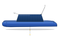
Three parameters carry the advance warning: the oxygen profile over depth, which shows how far depletion has progressed; phosphate in the deep water, which documents the release directly; and chlorophyll-a together with phycocyanin at the surface, which distinguish algal from cyanobacterial biomass. The WAMO 600 moves a probe package through the entire water column to a depth of 100 m and draws grab samples for the laboratory from the same layer. Secchi depth, turbidity and chlorophyll-a can additionally be derived from Sentinel-2 data for the surface of an entire lake; that is what SWIM does.
Which measure suits which stage depends on the lake, on the catchment and on whether the tipping point has already been passed. The measures catalogue orders 18 methods by effect and time frame, and the focus area water-body restoration describes the way back. The decision remains with the competent authority. The data on which it rests should come from depth and be gap-free.